How-To

How to Calculate Averages in Excel

By Ben Stockton

Published September 25, 2023

Calculating averages is a good way to learn more about your data in Excel. Learn how to calculate averages using Excel here.

There are plenty of reasons why you might want to calculate averages, whether it’s to make predictions, plan your budget, or track performance. You can also use the mean value of a set of data (or multiple data sets) to help you compare and contrast results.

To calculate averages in Excel, you can use a variety of functions to help you, including AVERAGE, SUM, COUNT, MEDIAN, and MODE. These functions help you to find the average results from your data without calculating it yourself.

If you want to know how to calculate averages in Excel, follow the steps below.

How to Calculate Averages in Excel with the AVERAGE Function

The AVERAGE function is a built-in function in Excel that allows you to calculate the average of a range of cells. It allows you to find the arithmetic mean value of a set of numbers. This is a useful way to help you understand trends or identify outliers in your data.

To use the AVERAGE function to calculate the average in Excel:

1. Open your Excel spreadsheet.
2. Select the cell where you want to display the average.
3. Type the formula =AVERAGE(
   
4. Next, type in or select the range of cells that you want to include in the average. For example, if you want to calculate the average of cells A2 to A10, you would enter “=AVERAGE(A2:A10)” (without quotation marks).
   
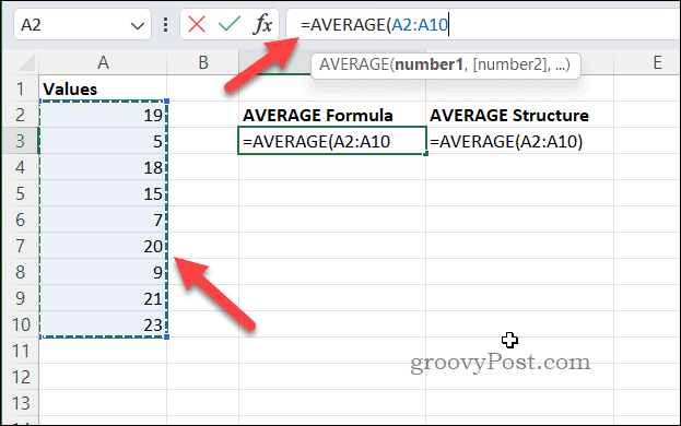
5. Press the Enter key to complete the formula. The selected cell will now display the average of the cell range.
   

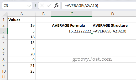
Note: You can also use the AVERAGE function to calculate the average of a selected range of cells by selecting the cells and then pressing AutoSum > Average in the Home tab on the ribbon.

The formula will be automatically entered into the selected cell and the average will be displayed.

How to Calculate Averages in Excel with the SUM/COUNT Formula

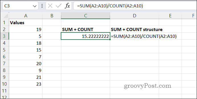
The SUM/COUNT formula is a simpler way to calculate the average of a range of cells in Excel. To use this method, you will need to add up all the values in the cell range using the SUM function and divide the total by the number of cells in the range using the COUNT function.

To calculate the average with the SUM/COUNT formula in Excel:

1. Select the cell where you want to display the result.
2. Using the formula bar, type =SUM( to begin the formula.
3. Select the cells that you want to include in the average or type in their cell ranges (e.g. =SUM(A2:A10) as the partial formula).
   
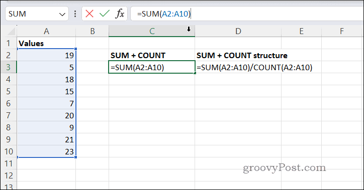
4. Type /COUNT( to complete the formula. (e.g. =SUM(A2:A10)/COUNT(
5. Select the cells that you want to include in the average again or type in the cell range (e.g. =SUM(A2:A10)/COUNT(A2:A10) as the full formula).
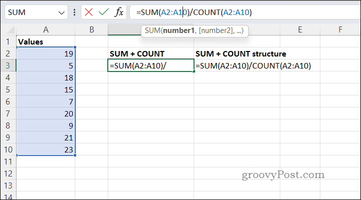
6. Press Enter on your keyboard to see the result.
   

How to Calculate the Median in Excel with the MEDIAN Function

The MEDIAN function is a built-in Excel function that allows you to easily calculate the median of a range of cells. The median is the middle value in a set of data, and it can be useful for understanding the central tendency of your data.

To calculate the median with the MEDIAN function in Excel:

1. Open your Excel spreadsheet.
2. Select the cell where you want to display the result.
3. On the formula bar, type =MEDIAN( to begin the formula.
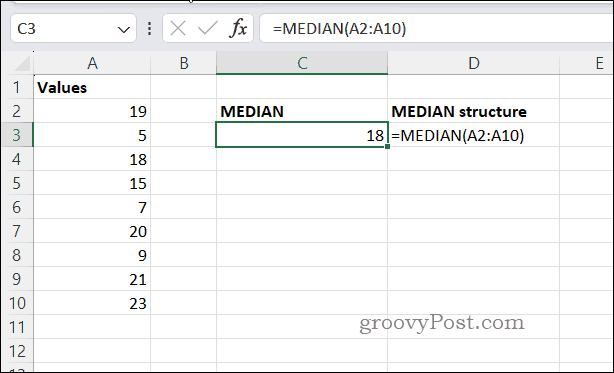
4. Next, select the cells you want to include or type in their cell range manually and close the formula with a final parenthesis (e.g. =MEDIAN(A2:A10) to use the cells from A2 to A10).
   
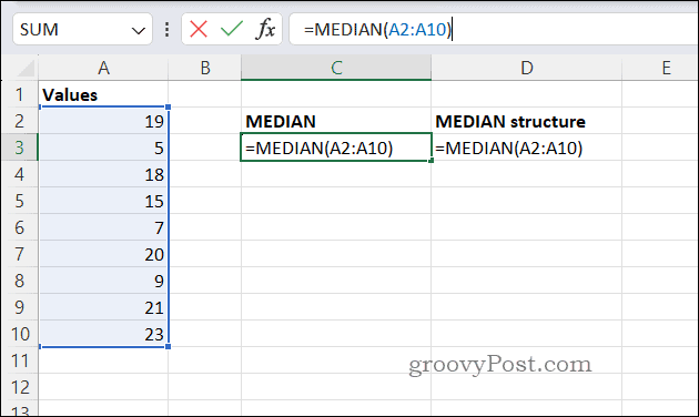
5. Press Enter to calculate the median result.
   

How to Calculate the Mode Values in Excel with the MODE Function

In mathematics, calculating the mode means identifying the most frequently occurring value in a data set. You can also calculate the mode value of a data set in Excel by using the MODE function to help you.

To calculate the mode value with the MODE function in Excel:

1. Open Excel.
2. Select the cell where you want to display the result.
3. Type =MODE( to begin the formula.
4. Select the cells that you want to include in the calculation or type in the cell range manually and type a closing parenthesis. For example, type =MODE(A2:A10) to calculate the mode from the values in cells A1 to A10.
   
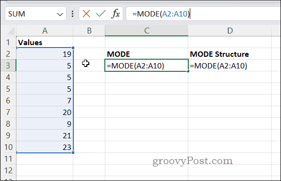
5. Press Enter to finish the formula and calculate the result.
   

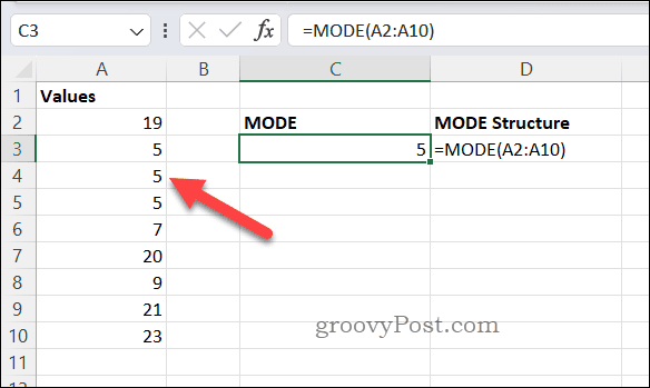
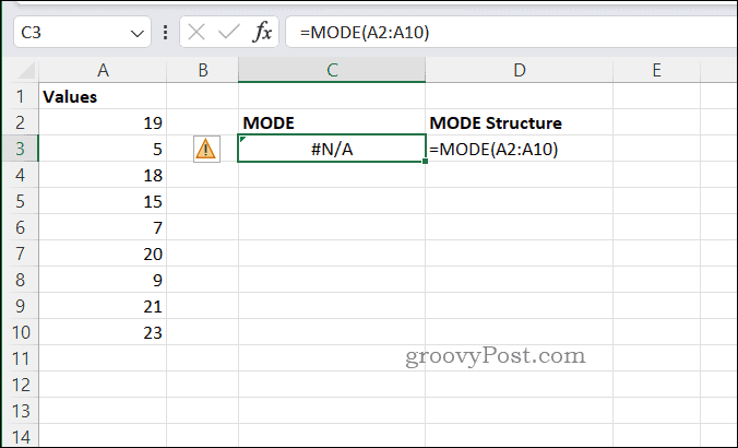
If the data set has more than one mode, the MODE function will return an array of all the modes. If the data set has no mode, the MODE function will return the #N/A error.

Analyzing Your Data in Excel

Thanks to the methods above, you can quickly and easily calculate the average of a range of cells in Excel. You can also calculate other statistical measures such as median, mean, and mode using similar functions.

There are many other tips and tricks that Excel users should know to work efficiently and effectively with their data. For example, you can learn how to ignore errors in Excel to help you bypass any expected mistakes. You can also speed up your spreadsheet performance by replacing a formula with the result it generates.

You may also want to learn how to work with comments and notes in Excel to add context and clarity to your data.