How-To

How to Extract Text From a Cell in Excel

By Ben Stockton

Published September 25, 2023

Are you looking to extract text from a cell in Microsoft Excel? This guide walks you through using the LEFT, RIGHT, MID, or FIND functions to do that.

Microsoft Excel extends far beyond simple data entry and analysis. You can use it to create complex spreadsheets that allow you to sort through huge data sets. You can use spreadsheets to perform difficult calculations, create graphs, and more.

However, some of Excel’s more basic functions can be equally useful when it comes to organizing and managing data. If you’re trying to extract text from a cell in Excel, there are several methods you can use to achieve this.

Here are some ways you can extract text from a cell in Microsoft Excel.

Using LEFT, MID, and RIGHT Functions

To extract text from a cell in Excel, you can use one of several built-in functions, such as the LEFT, MID, or RIGHT functions.

Each of these three functions extracts a specific number of characters from a text string. This can either be from a cell (using cell references) or from a string in the formula itself. The names (LEFT, RIGHT, and MID) refer to the starting points.

For instance, if you use LEFT, you would identify the number of characters starting from the left that you’d like to save. Likewise, using RIGHT, the number and position of characters would start from the right.

Creating a Formula Using LEFT or RIGHT

To begin, open your Excel spreadsheet, select an empty cell, and click the formula bar so that the blinking cursor is active. From there, you can type your formula. Both LEFT and RIGHT functions follow the same pattern. For example:

=LEFT(text,character_number) or =RIGHT(text,character_number)

• Replace text with either a text string (in quote marks) or a cell reference.
• Replace character_number with the number of characters you want to extract, starting from the furthest left or right position.

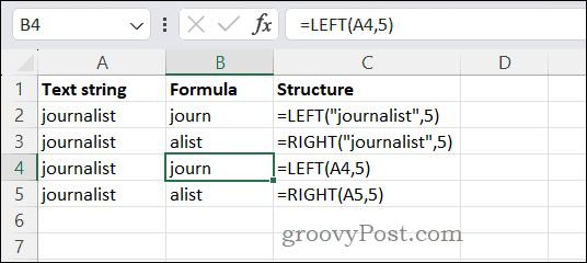
For example, to extract the first five characters from the word journalist using LEFT, you’d type:

=LEFT("journalist",5)

Likewise, to extract the last five characters using RIGHT, you’d type:

=RIGHT("journalist",5)

If the word journalist was in cell A4, you’d type the following for LEFT:

=LEFT(A4,5)

For RIGHT (assuming the word journalist was in cell A5), you’d type the following instead:

=RIGHT(A5,5)

Creating a Formula Using MID in Excel

The MID function in Excel works in the same way, but you’ll have an extra argument to consider. To use MID, use this structure:

=MID(text,start_number,character_number)

• As with LEFT or RIGHT, text refers to a text string or cell reference.
• Replace start_number with the position in the text string you want to start counting.
• Replace character_number with the number of characters to count and extract.

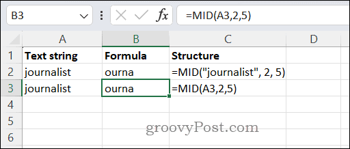
To extract five characters after the first two characters in the word journalist, you’d use

=MID("journalist", 2, 5)

If the word was in cell A3, you’d type:

=MID(A3,2,5)

The value returned can then be analyzed or used in other parts of your spreadsheet.

Using the FIND Function in Excel

The FIND function in Excel is used to locate the place of a character number within a text string. You can use this to extract text based on a pattern or search criteria. The FIND function uses this structure and syntax:

=FIND(text_search,text,start_number)

• In this formula, text_search refers to the search criteria you’re looking for. If you want to extract a certain word, type it here, or you could type a letter. You can type a search string into the formula directly or refer to a cell reference that contains a text string. If you type the string into the formula directly, make sure to wrap it in quotation marks.
• The text argument refers to the string you’re analyzing—this is what FIND will take its characters from. You could type a string directly here (wrapped in quote marks) or use a cell reference that contains a text string.
• Finally, start_number indicates where in the text string FIND should start. Like LEFT, RIGHT, and MID, this is based on the number of characters, starting from the left.

Here’s an example. Let’s assume that cell A2 has a search query (dog), cell B2 has a text string (The dog’s name is Bill and he’s a good dog.), and the starting number is 9. There are two examples of the word dog in this query, so the possible results could be either 5 or 40, depending on your starting number.

Here’s an example formula:

=FIND(A2,B2,9)

If the query and text strings are used in the formula directly, you’d use this formula instead:

=FIND("dog","The dog's name is Bill and he's a good dog.",9)

In both cases, FIND will return 40.  There’s only one dog that counts–that’s the second one in the string. Because the starting number is 9, the first example of dog in the string is too early for it to count. In the third row, however, we’ve left out the starting character. Therefore, the formula returns 5, the first instance of dog in the example.

Using Excel for Data Analysis

You can quickly extract text from a cell in Excel using the steps above. If you’re starting out as a data analyst, extracting text from cells is a useful skill that can help you manipulate your data and remove anything extraneous.